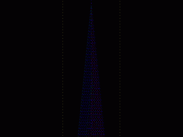
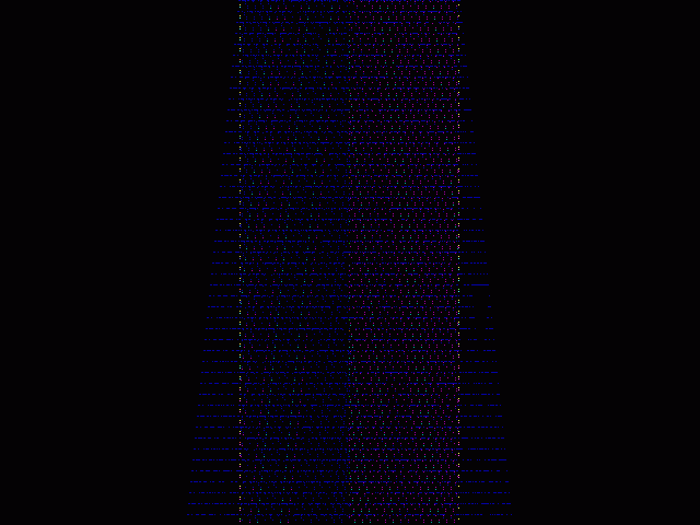
Fig. 1: The evolution of EPR CA from generation 0. Distance to detectors from source C is 100 cells wide.
Last revised: May 07, 2005, 2:33 PM.
In the present work we shall construct a classical (i.e. non-quantum) cellular automaton that will be able to produce (we suppose, for a great surprise of many) truly quantum (!) mechanical (namely, EPR) effects. Thus, we shall demonstrate clearly (by giving a concrete example) that the theorem proven by J. S. Bell in 1964 [Bel64] has nothing to do with otherwise purely local and deterministic mathematical models like CAs.
The example we have in mind is a simple one-dimensional CA. We shall construct this 1D CA from a few other 1D CAs, i.e. our "EPR CA" is actually a superposition of many 1D CAs specially made for our task.
Below we shall rely heavily on the well-known work of N. David Mermin [Mer85].
While any other EPR paper can be used, we have decided to choose [Mer85] for its unprecedented quality of presentation and explanation. This work has inspired much research in today's quantum computation field and has the unique feature of being readable for both theoretical physicists and theoretical computer scientists.
(Instead of the original EPR [EPR35] and Bell's [Bel64] papers we would also like to recommend [Esp79]. In that work, the proof of Bell's theorem given by d'Espagnat is rather easy to follow. In any case, [Mer85] is the only reference one needs in order to fully understand the contents of the present article; no knowledge of quantum mechanics or cellular automata theory is required.)
For the convenience of our reader, in the next section we shall outline briefly the main ideas of Mermin's classic cited above.
In his work [Mer85] N. David Mermin proposes a gedanken (thought) experiment that is a somewhat simplified version of the real physical experiments held in a laboratory (for example, one can think about famous EPR experiments of Aspect et al. [AGR82, ADR82]).
The experimental setup proposed by Mermin consists of three pieces: two of them (A and B) function as detectors, and the third piece (C), midway between A and B, functions as a source of something ("particles" or whatever).
Detectors A and B are far apart from each other (in the analogous Aspect experiments - more than 10 meters apart). Each detector has a switch that can be set to one of three possible positions (to be recorded below as '1', '2' or '3'). Also, each detector responds to an event (passage of a "particle" from C to that detector) by flashing either a green light (to be denoted as 'G') or a red one ('R').
The switches of the detectors are independently and randomly set to one of its positions, and two "particles" are emitted simultaneously from the source C to detectors A and B, respectively. Shortly after that, each detector flashes either green or red. The settings of the switches are recorded, as well as the flashes of the lamps, and then the whole experiment is repeated many times.
The data obtained from each separated run is recorded as something like '32RG', where '3' in this example denotes the setting of the switch at detector A, '2' - the setting of the switch at detector B, 'R' denotes the red flash of A, and 'G' - the green flash obtained from detector B, respectively.
Typical data from a large number of runs is shown in Table 1 below.
| Run # | Result |
| 1 | 31RG |
| 2 | 33GG |
| 3 | 33RR |
| 4 | 12GR |
| 5 | 33GG |
| 6 | 21GR |
| 7 | 21RR |
| 8 | 22RR |
| 9 | 33GG |
| 10 | 11GG |
| 11 | 23RR |
| 12 | 32GR |
| 13 | 12GR |
| 14 | 12RG |
| 15 | 11GG |
| 16 | 31RG |
| 17 | 12RG |
| 18 | 13GR |
The data obtained has the following two relevant features:
The rest of the paper Mermin devotes to showing why one should be bothered by such results and why they violate the famous inequality/theorem proven by J. S. Bell in 1964.
Applying Bell's theorem, it is easy to deduce that if the settings of the switches are random then the same colors will flash at least 5/9 of all the runs, i.e. the second feature of the data will be irreproducible.
Mermin concludes his work by showing how the same data, nevertheless, is obtained in a real EPR experiment. "One way to do it" -- writes Mermin -- is to use some quantum mechanical "magic" in the form of Stern-Gerlach magnets and particles with spin ½ in a singlet state.
The present article has the ambitious task to show to "anybody who is bothered" by Bell's theorem that the same result, however, could be obtained in a completely mechanical system. (As we have shown in our work [Pet02f], all kind of cellular automata are mechanically constructible systems that are able to show synchronous behavior without actually synchronizing themselves).
And anybody who thinks there is no way to reproduce these results for cellular automata has to have "rocks in his head"1, especially if he believes there is some connection between Bell's theorem and cellular automata.
The simple truth is that Bell's theorem can not be applied to CAs, at least not directly. The domain of the theorem is irrelevant to cellular automata, therefore there is no way one can make the "conclusion" that EPR effects are unobtainable in a CA "because of Bell's theorem" (an opinion that has been commonly accepted in some physicists circles for a long time).
While the very fact that Bell's theorem is not applicable to CAs is indisputable, one may still doubt that, despite this, cellular automata can be able to serve as good mathematical models for some certain quantum mechanical phenomena that seem so weird to our senses& But they can!
We shall proceed our exposition by showing a concrete CA that is able to produce real EPR effects. To explain what we have in mind, we need to translate all the usual physics terminology into CA terms. For a non-expert in the field of cellular automata this may seem a little bizarre at first, but actually the whole thing is much simpler than any QM "explanation" ever made.
We shall supply our exposition with a lot of pictures and statistical data, so we are certain our CA based model will quickly begin to make sense for our reader, whether he is a theoretical physicist or theoretical computer scientist.
Actually, yet another simple truth is that QM does not explain EPR; it merely computes the final result. So the very fact that we shall be able to demonstrate a clear mathematical model that reproduces also the mid-steps toward generating EPR effects, not just the statistical data at the end of the experiment, should be regarded, we hope, as more or less remarkable even by the most ardent worshipers of QM.
Cellular automata are dynamic complex systems composed of small discrete elements ("cells") that operate synchronously in time accordingly to some local function ("rule").
It is important to emphasize that all cells can take values from some fixed set of discrete elements ("states"), and time operates in discrete intervals we call "steps". In other words, physically speaking: for CAs space and time are completely discrete, and their rules of Nature are deterministic.
For the special purpose of this article we shall need to study only the simplest form of CAs called one-dimensional cellular automata. For them, space can be thought to be an infinite row of adjacent cells.
We usually denote cells of a 1D CA with c(x, t), where x and t are integers representing the spatial position of some cell c and the time step number, respectively. For binary CAs, c(x, t)Î{0, 1}, i.e. all cells can take only two possible values.
Now, we need to translate the usual physics terminology from [Mer85] into CA terms. First of all, let us think of some spatially distant positions a and b that shall represent the positions of detectors A and B, respectively.
To represent adequately what is happening for each detector we need to represent somehow the position of the switch and the state of the lights for that detector. Therefore, let us say that each detector can have an internal state that is composed by the position of its switch ('0' -- switch not set yet, '1' -- switch set to position 1, '2' -- switch set to position '2', and '3' -- switch set to position 3) and the state of the lights ('0' -- no flash, '1' -- green flash, '2' -- red flash).
Thus, each detector can take 4*3=12 states.
Let us think now that our one-dimensional CA has some sufficiently large number of states per cell (namely, at least 12 states per cell). We can say these 12 states actually represent two groups of substates: one of them (4 states) representing the switches, the other one (3 states) -- the state of the lights.
Probably it will be best to think of two "sub-cells", for example a=
Since we want to demonstrate EPR effects for this CA, we shall need the sub-cells that represent the positions of switches of the two detectors (namely, a1 and b1) to change their states randomly during the evolution of the CA.
To represent the two key features of Mermin's though experiment (cf. Section 2) we need to have the following:
And that is all we need to represent EPR correlations for some CA!
The next section of our work is a detailed description of the rule of a concrete example of EPR CA. For all readers not familiar with cellular automata we strongly recommend downloading our software2 and running it first (in order to get the "look and feel" of how the whole thing works) before proceeding any further with this article.
Our EPR CA is a 1D CA with 2*3*2*8*4*4*3*4=18432 states. Each cell of this CA has one neighbor on its left and right side, i.e. this is a (18432, 1) one dimensional CA, using Wolfram's notation.
The rule of this CA can be described as a function f that operates over the cells c of the CA in the following form:
Since here every cell can take 18432 states, to simplify the rule description, we shall represent each x as an ordered octet:
where:
i.e. c(x1,t) is a bit, c(x2,t) is a trit, c(x3,t) is a bit again, c(x4,t) can take 8 states, etc.
We shall depict these substates as 8 different lines (rows).
For clarity, let us call these lines as follows:
x1 -- Rule 30 line
x2 -- Particle direction line
x3 -- Particle spin line
x4 -- Source C line
x5 -- Detector lights state line
x6 -- Detector switch state line
x7 -- Virtual particle direction line
x8 -- Virtual particle parameter line
To work properly, EPR CA must have initial configuration of this kind:
........1........ Rule 30 line
................. Particle direction line
................. Particle spin line
........1........ Source C line
...1.........1... Detector lights state line
................. Detector switch state line
................. Virtual particle direction line
................. Virtual particle parameter line
(On the textual diagram above the distance to detectors from source C is 5, but it may be set arbitrarily large. Also, all dots here represent zeros, while dots used on the diagrams below represent "any state")
Let us denote the change of the state of some cell c(xi, t) and the state of its neighbors c(xi-1, t) and c(xi+1, t) with the following rule transition:
c(x1-1,t) c(x1,t) c(x1+1,t) => c(x1,t+1)
... => ...
c(x8-1,t) c(x8,t) c(x8+1,t) => c(x8,t+1)
Now, we can describe the rule of the EPR CA by saying that:
except the following cases...
Rule 30 description:
001 => 1 Rule 30 line
... => . Particle direction line
... => . Particle spin line
... => . Source C line
... => . Detector lights state line
... => . Detector switch state line
... => . Virtual particle direction line
... => . Virtual particle parameter line
010 => 1 Rule 30 line
... => . Particle direction line
... => . Particle spin line
... => . Source C line
... => . Detector lights state line
... => . Detector switch state line
... => . Virtual particle direction line
... => . Virtual particle parameter line
011 => 1 Rule 30 line
... => . Particle direction line
... => . Particle spin line
... => . Source C line
... => . Detector lights state line
... => . Detector switch state line
... => . Virtual particle direction line
... => . Virtual particle parameter line
100 => 1 Rule 30 line
... => . Particle direction line
... => . Particle spin line
... => . Source C line
... => . Detector lights state line
... => . Detector switch state line
... => . Virtual particle direction line
... => . Virtual particle parameter line
(The middle random bit of Rule 30 is used as a pseudo-random number generator - see below)
Source C changes its "internal" state from 1 to 7 and then back to 1:
... => . Rule 30 line
... => . Particle direction line
... => . Particle spin line
.x. => y Source C line
... => . Detector lights state line
... => . Detector switch state line
... => . Virtual particle direction line
.z. => z Virtual particle parameter line
where y=x+1 for xÎ{1,...,6} and y=1 for x=7.
(Also, please note that the virtual particle parameter is preserved)
Detector changes state back to inactive ('1'), if activated:
... => . Rule 30 line
... => . Particle direction line
... => . Particle spin line
... => . Source C line
.x. => 1 Detector lights state line
.y. => y Detector switch state line
... => . Virtual particle direction line
... => . Virtual particle parameter line
where x>0. Note also that detector's switch state is preserved.
Source C memorizes the random bit state at particle spin position, if C=1:
.x. => . Rule 30 line
... => . Particle direction line
... => x Particle spin line
.1. => 2 Source C line
... => . Detector lights state line
... => . Detector switch state line
... => . Virtual particle direction line
.z. => z Virtual particle parameter line
Source C memorizes the random bit state at particle spin position, if C=3:
.x. => . Rule 30 line
... => . Particle direction line
... => x Particle spin line
.3. => 4 Source C line
... => . Detector lights state line
... => . Detector switch state line
... => . Virtual particle direction line
.z. => z Virtual particle parameter line
Source C memorizes the last left traveling virtual particle parameter, if C=2:
.x. => . Rule 30 line
... => . Particle direction line
.y. => . Particle spin line
.2. => 3 Source C line
... => . Detector lights state line
... => . Detector switch state line
... => . Virtual particle direction line
... => z Virtual particle parameter line
where z=2y+x.
Source C emits right traveling virtual particle:
x.. => . Rule 30 line
... => . Particle direction line
y.. => . Particle spin line
4.. => . Source C line
... => . Detector lights state line
... => . Detector switch state line
... => 2 Virtual particle direction line
... => z Virtual particle parameter line
where z=2y+x.
Source C emits left traveling virtual particle:
..x => . Rule 30 line
... => . Particle direction line
..y => . Particle spin line
..2 => . Source C line
... => . Detector lights state line
... => . Detector switch state line
... => 1 Virtual particle direction line
... => z Virtual particle parameter line
where z=2y+x.
Source C memorizes the comparison of last virtual particle parameters, if C=5:
.x. => . Rule 30 line
... => . Particle direction line
... => s Particle spin line
.5. => 6 Source C line
... => . Detector lights state line
... => . Detector switch state line
... => . Virtual particle direction line
.zy => x Virtual particle parameter line
where s=1, if z=y, else s=0.
Source C accumulates Rule 30 bit states for later usage, if C=6:
.x. => . Rule 30 line
... => . Particle direction line
.y. => y Particle spin line
.6. => 7 Source C line
... => . Detector lights state line
... => . Detector switch state line
... => . Virtual particle direction line
.z. => s Virtual particle parameter line
where s=2x+z.
Right traveling particle on the left:
... => . Rule 30 line
2.. => 2 Particle direction line
x.. => x Particle spin line
... => . Source C line
.0. => . Detector lights state line
... => . Detector switch state line
... => . Virtual particle direction line
... => . Virtual particle parameter line
Detector flashes, if right traveling particle detected and switch has been set:
... => . Rule 30 line
2.. => . Particle direction line
x.. => . Particle spin line
... => . Source C line
.y. => z Detector lights state line
.s. => s Detector switch state line
... => . Virtual particle direction line
... => . Virtual particle parameter line
where z=x+2, if y>0 and s>0.
Left traveling particle on the right:
... => . Rule 30 line
..1 => 1 Particle direction line
..x => x Particle spin line
... => . Source C line
.0. => . Detector lights state line
... => . Detector switch state line
... => . Virtual particle direction line
... => . Virtual particle parameter line
Detector flashes, if left traveling particle detected and switch has been set:
... => . Rule 30 line
..1 => . Particle direction line
..x => . Particle spin line
... => . Source C line
.y. => z Detector lights state line
.s. => s Detector switch state line
... => . Virtual particle direction line
... => . Virtual particle parameter line
where z=x+2, if y>0 and s>0.
Right traveling virtual particle on the left:
... => . Rule 30 line
... => . Particle direction line
... => . Particle spin line
... => . Source C line
.0. => . Detector lights state line
... => . Detector switch state line
2.. => 2 Virtual particle direction line
x.. => x Virtual particle parameter line
Sets detector's switch, if right traveling virtual particle detected:
... => . Rule 30 line
... => . Particle direction line
... => . Particle spin line
... => . Source C line
.y. => y Detector lights state line
... => x Detector switch state line
2.. => . Virtual particle direction line
x.. => . Virtual particle parameter line
where y>0.
Left traveling virtual particle on the right:
... => . Rule 30 line
... => . Particle direction line
... => . Particle spin line
... => . Source C line
.0. => . Detector lights state line
... => . Detector switch state line
..1 => 1 Virtual particle direction line
..x => x Virtual particle parameter line
Sets detector's switch, if left traveling virtual particle detected:
... => . Rule 30 line
... => . Particle direction line
... => . Particle spin line
... => . Source C line
.y. => y Detector lights state line
... => x Detector switch state line
..1 => . Virtual particle direction line
..x => . Virtual particle parameter line
where y>0.
Source C emits right traveling particle with spin=x:
x.. => . Rule 30 line
... => 2 Particle direction line
1.. => x Particle spin line
7.. => . Source C line
... => . Detector lights state line
... => . Detector switch state line
... => . Virtual particle direction line
... => . Virtual particle parameter line
Source C emits right traveling particle with spin=0 (i.e. "spin down"):
0.. => . Rule 30 line
... => 2 Particle direction line
0.. => 0 Particle spin line
7.. => . Source C line
... => . Detector lights state line
... => . Detector switch state line
... => . Virtual particle direction line
0.. => . Virtual particle parameter line
Source C emits right traveling particle with spin=0:
0.. => . Rule 30 line
... => 2 Particle direction line
0.. => 0 Particle spin line
7.. => . Source C line
... => . Detector lights state line
... => . Detector switch state line
... => . Virtual particle direction line
1.. => . Virtual particle parameter line
Source C emits right traveling particle with spin=0:
0.. => . Rule 30 line
... => 2 Particle direction line
0.. => 0 Particle spin line
7.. => . Source C line
... => . Detector lights state line
... => . Detector switch state line
... => . Virtual particle direction line
2.. => . Virtual particle parameter line
Source C emits right traveling particle with spin=0:
0.. => . Rule 30 line
... => 2 Particle direction line
0.. => 0 Particle spin line
7.. => . Source C line
... => . Detector lights state line
... => . Detector switch state line
... => . Virtual particle direction line
3.. => . Virtual particle parameter line
Source C emits right traveling particle with spin=1 (i.e. "spin up"):
1.. => . Rule 30 line
... => 2 Particle direction line
0.. => 1 Particle spin line
7.. => . Source C line
... => . Detector lights state line
... => . Detector switch state line
... => . Virtual particle direction line
0.. => . Virtual particle parameter line
Source C emits right traveling particle with spin=1:
1.. => . Rule 30 line
... => 2 Particle direction line
0.. => 1 Particle spin line
7.. => . Source C line
... => . Detector lights state line
... => . Detector switch state line
... => . Virtual particle direction line
1.. => . Virtual particle parameter line
Source C emits right traveling particle with spin=1:
1.. => . Rule 30 line
... => 2 Particle direction line
0.. => 1 Particle spin line
7.. => . Source C line
... => . Detector lights state line
... => . Detector switch state line
... => . Virtual particle direction line
2.. => . Virtual particle parameter line
Source C emits right traveling particle with spin=1:
1.. => . Rule 30 line
... => 2 Particle direction line
0.. => 1 Particle spin line
7.. => . Source C line
... => . Detector lights state line
... => . Detector switch state line
... => . Virtual particle direction line
3.. => . Virtual particle parameter line
Source C emits left traveling particle with spin=x:
..x => . Rule 30 line
... => 1 Particle direction line
..1 => x Particle spin line
..7 => . Source C line
... => . Detector lights state line
... => . Detector switch state line
... => . Virtual particle direction line
... => . Virtual particle parameter line
Source C emits left traveling particle with spin=0:
..0 => . Rule 30 line
... => 1 Particle direction line
..0 => 0 Particle spin line
..7 => . Source C line
... => . Detector lights state line
... => . Detector switch state line
... => . Virtual particle direction line
..0 => . Virtual particle parameter line
Source C emits left traveling particle with spin=1:
..0 => . Rule 30 line
... => 1 Particle direction line
..0 => 1 Particle spin line
..7 => . Source C line
... => . Detector lights state line
... => . Detector switch state line
... => . Virtual particle direction line
..1 => . Virtual particle parameter line
Source C emits left traveling particle with spin=1:
..0 => . Rule 30 line
... => 1 Particle direction line
..0 => 1 Particle spin line
..7 => . Source C line
... => . Detector lights state line
... => . Detector switch state line
... => . Virtual particle direction line
..2 => . Virtual particle parameter line
Source C emits left traveling particle with spin=1:
..0 => . Rule 30 line
... => 1 Particle direction line
..0 => 1 Particle spin line
..7 => . Source C line
... => . Detector lights state line
... => . Detector switch state line
... => . Virtual particle direction line
..3 => . Virtual particle parameter line
Source C emits left traveling particle with spin=0:
..1 => . Rule 30 line
... => 1 Particle direction line
..0 => 0 Particle spin line
..7 => . Source C line
... => . Detector lights state line
... => . Detector switch state line
... => . Virtual particle direction line
..0 => . Virtual particle parameter line
Source C emits left traveling particle with spin=0:
..1 => . Rule 30 line
... => 1 Particle direction line
..0 => 0 Particle spin line
..7 => . Source C line
... => . Detector lights state line
... => . Detector switch state line
... => . Virtual particle direction line
..1 => . Virtual particle parameter line
Source C emits left traveling particle with spin=0:
..1 => . Rule 30 line
... => 1 Particle direction line
..0 => 0 Particle spin line
..7 => . Source C line
... => . Detector lights state line
... => . Detector switch state line
... => . Virtual particle direction line
..2 => . Virtual particle parameter line
Source C emits left traveling particle with spin=1:
..1 => . Rule 30 line
... => 1 Particle direction line
..0 => 1 Particle spin line
..7 => . Source C line
... => . Detector lights state line
... => . Detector switch state line
... => . Virtual particle direction line
..3 => . Virtual particle parameter line
In order to represent adequately the dynamics of EPR CA, we shall need some color presentation. For better visibility, we shall represent the state of the Rule 30 line, the internal state of the source C, and all moving particles with dark (non-intensive) colors, while the state of the detectors (lights + switch) will be depicted with bright (intensive) colors.
In other words: we shall represent all micro ("quantum") level events taking place in our CA (movement of the particles, changes of the internal state of source C) with dark colors, while all macro level events (flashes of the detectors, settings of the switches) will be represented with bright colors.
The following table represents the association between the (sub-)states and colors used (cf. Section 5):
| Line name \ Cell state |
|
|
|
|
|
|
|
|
| Rule 30 line |
|
|
||||||
| Particle direction line |
|
|
|
|||||
| Particle spin line |
|
|
||||||
| Source C line |
|
|
|
|
|
|
|
|
| Detector lights state line |
|
|
|
|
||||
| Detector switch state line |
|
|
|
|
||||
| Virtual particle direction line |
|
|
|
|||||
| Virtual particle parameter line |
|
|
|
|
Below we shall provide some color pictures of the evolution of EPR CA.
Below we provide some statistical data produced by the software realization of EPR CA for generations number 5000, 10000 and 15000. As we shall see, in all three cases tested our CA violates Bell's inequality that predicts the number of the same flashes must be at least 5/9 of all runs.
Statistical data for all possible combinations of switches/flashes generated for the first 5,000 time steps of EPR CA evolution is shown in Table 3 below:
|
|
|
|
|
|
|
|
|
|
|
|
|
|
|
|
|
|
|
|
|
|
|
|
|
|
|
|
|
|
|
|
|
|
|
|
|
|
|
|
|
|
|
|
|
|
|
|
|
|
|
|
|
|
|
|
|
|
|
|
|
|
|
|
|
|
|
|
|
|
|
|
|
|
|
|
|
Same flashes (GG+RR)=173, different flashes (RG+GR)=199
For generation 5000 the number of different flashes is actually greater than the number of the same flashes, so here clearly we have a situation when Bell's inequality is violated.
Statistics for the switches/flashes generated is shown in table 4:
|
|
|
|
|
|
|
|
|
|
|
|
|
|
|
|
|
|
|
|
|
|
|
|
|
|
|
|
|
|
|
|
|
|
|
|
|
|
|
|
|
|
|
|
|
|
|
|
|
|
|
|
|
|
|
|
|
|
|
|
|
|
|
|
|
|
|
|
|
|
|
|
|
|
|
|
|
Same flashes (GG+RR)=393, different flashes (RG+GR)=393
This particular result is impressive with the fact that here we have an exact match with the second feature of the data as required by Mermin's gedanken experiment: the number of the runs in which lights flash the same color is exactly the same as the number of the runs in which lights flash different colors!
Statistics for the switches/flashes generated is shown in Table 5:
|
|
|
|
|
|
|
|
|
|
|
|
|
|
|
|
|
|
|
|
|
|
|
|
|
|
|
|
|
|
|
|
|
|
|
|
|
|
|
|
|
|
|
|
|
|
|
|
|
|
|
|
|
|
|
|
|
|
|
|
|
|
|
|
|
|
|
|
|
|
|
|
|
|
|
|
|
Same flashes (GG+RR)=614, different flashes (RG+GR)=596
Although here the number of the same flashes is greater than the number of different flashes, still it is a fraction very close to 50% (to be exact, 50.74%) of all runs. Since 5/9=55.55% then in this case we have a result that violates Bell's inequality as well, and therefore is in full concordance with quantum mechanics.
It is easy to check out that our classical (non-quantum) CA generates quantum mechanical (EPR) effects similar to these described in [Mer85].
So, what is the whole trick?!
Probably the best short answer to this question will be: there is no trick; the EPR CA simply works, and works properly.
A more elaborate answer, however, might be:
The "trick" is that actually the positions of the switches at detectors A and B are not random, they are pseudo-random. But: pseudo-randomness is something essentially different from (true) randomness!
Immediately when one recognized the difference between the two notions, one starts to realize that what is going on at position A is not, at least, necessarily independent from what is happening at position B. For if one can use a pseudo-random number generator (PRNG) to produce a temporary sequence of states for point A, then there is no problem for the same sequence to be generated in a spatially distant point B as well, if one knows what the formula (PRNG) is used for generating the sequence at A.
For cellular automata, there is simply no such thing as "true randomness": they are completely deterministic computational models. For CAs, what is happening at point A is always related to what happened (and is happening) at point B, and there is simply no way to get rid of these correlations, even if one wants to do so.
Now that we have revealed that the key feature essential for this CA to work is pseudo-randomness, we can say that the rest of the "assembly work" done to make such a CA is just a matter of good mathematical technique and a little bit of creativity.
To be quite honest, we can reveal also that in our somewhat simplified example the settings of the switches are actually generated (!) by the source C itself!
(Let this statement serve as a small "hint" for all CA experts and enthusiasts& However, we shall leave the rest of the "reverse engineering" of how and why EPR CA works for the reader. We can add only that we are certain that EPR CA will work for any larger number of runs, and we actually do not need to "test" it statistically, i.e. the success of the "computational experiments" done with this CA is guaranteed by its very construction&)
Anyway, much more clever CA models of this kind can be constructed (something that will generate the settings of the switches outside the source C, for example). But this is not necessary.
The important point here is that, mathematically speaking, Bell's theorem is not at all an obstacle for any classical (i.e. non-quantum) CA to demonstrate EPR effects of any kind!
(The author of the present article is ready to demonstrate CA-based mathematical models for any known physical experiment of EPR effects, regardless of how "clever" the experiment is. This may include computational experiments with 3D CAs instead of 1D CAs, any proper timing, detectors that use more than 3 states per switch, etc. But, again: all this is not at all important!)
The important point of the whole story can be summarized as follows:
Bell's theorem is simply irrelevant to cellular automata.
The restriction proposed by J. S. Bell with his famous inequality may be something that shocks physicists traditionally operating with notions like "continuity" and "randomness", but it is not at all a problem for perfectly local and deterministic mathematical models like CAs that replace these notions with the corresponding notions of finitely divisible space/time and pseudo-randomness.
Why is all of this important?!
Well, there is a long story behind the basic demonstration of our current work, but if we have to summarize it very briefly, it could be described as follows...
In the 1960s Edward Fredkin [Gar71, Fre90] and, independently, Konrad Zuse [Zus67, Zus69] proposed the idea that our Universe is a three-dimensional cellular automaton. The idea that the Universe is a CA is now known as the "Zuse-Fredkin thesis", and the emerging new scientific field as "Digital Physics" (DP).
In 2002 Stephen Wolfram exploited the same idea by publishing a hefty (1200 pages) volume called "A New Kind of Science" (NKS) [Wol02]. This work may have its good points and bad (in particular, Wolfram has been criticized for his self-advertising style and for not giving enough credit to Fredkin and Zuse), but the fact is that quickly after its publication NKS become a bestseller.
Digital Physics is now recognized as one of the branches of the so-called "Physics of Computation" -- a mix between theoretical physics and theoretical computer science.
Since DP is heavily built on cellular automata theory, there is no surprise that two of the basic postulates of DP are that space-time is discrete and that the laws of physics are deterministic.
While the ideas of Digital Physics may seem quite odd from the viewpoint of contemporary physics, they have a stable basis in theoretical computer science (CS) and metamathematics [Pet02a1, Pet02a2].
For example, from metamathematics we know that the very process of doing mathematics is nothing but the manipulation of a finite number of symbols (i.e. finite set of discrete elements) using discrete steps while transforming one mathematical equation into another. Hence the appearance of discrete space and time.
Full determinism is a consequence of the fact that mathematical reasoning (i.e. theorem proving) is always a strictly causal process and never "random".
Similarly, in theoretical CS we use the so-called "Church-Turing thesis". According to that thesis, all mathematical functions can be computed on a (somewhat primitive) serial computational device known as a "Universal Turing Machine" (UTM) [Tur36]. Since all of theoretical physics relies on mathematical functions and models, there is no surprise that our Universe must be some kind of computer [Pet02a1]. If it is not, then the pursuit of a purely mathematical formulation of physics is in vain, since all human machines (scientists) are subject to the constraints of finiteness and discreteness. (i.e. If the universe is not some kind of computer, then human beings have no possibility of realizing its precise nature since finite and discrete reasoning is the only tool of discovery available to them!)
While UTMs fully encompass the whole spectrum of mathematical functions and models in terms of "computability", there is still some room for "improvement" in the computational model: the problem is that UTMs are serial devices and they are quite slow in computing some functions, while CAs allow parallel computation and they are significantly "faster" [Pet02a2].
The question now is: how fast can the fastest computational device be?
Since 1985 there has been increasing interest in exploring various phenomena in quantum physics, like EPR and parallelism on the quantum level. Some even suggest that our Universe is not exactly a (classical) CA, but a quantum CA.
But hailing the brand new field of "quantum computation" (QC) may be premature.
While QC may seem quite attractive for the human imagination, it is worth noticing that the theoretical basis of quantum physics is the same old mathematics that works well on fully mechanical computational devices like UTMs and (classical) CAs [Pet02a2]. Regardless of the "continuous" and "probabilistic" notions that modern physicists manipulate with pencil and paper, they are still confined to working with a finite number of symbols -- within a finite amount of time -- in a discrete number of steps. There simply is no ways around this.
And as if that weren't enough, we have clearly demonstrated in the present work, that the phenomenon of EPR works quite well for classical CAs, so there simply is no need for unbiased enthusiasm.
The important thing to be understood here is that Digital Physics attacks the very foundation of quantum mechanics, as we know it. Hence, from the viewpoint of DP, the very use of QM as a "scientific basis" for QC is unacceptable.
DP replaces one of the basic postulates of QM ("true randomness") with another one (determinism, i.e. pseudo-randomness). For significantly complex systems (like computationally universal cellular automata) pseudo-randomness is essentially indistinguishable from the (true) randomness.
In its essence, Digital Physics is a proposal for a paradox-free science; it is a proposal to rebuild the whole foundation of physics on a stable ground.
DP has already successfully explained some centuries-old metaphysical paradoxes like those of Zeno (450 B.C.). For example, the well-known paradox of Achilles "eternally chasing" the turtle is resolved in DP by simply noticing the fact that (for cellular automata) both space and time are discrete (not continuous), and therefore they are not infinitely divisible [Pet02a2].
As we demonstrated in the present work, DP explains the EPR paradox by effectively replacing one of the QM postulates (the belief that the world "at the bottom" is essentially random) with another one (the laws of Nature are deterministic, and the quantum world is pseudo-random).
Yet another simple truth is that QM actually does not actually explain the EPR paradox at all; QM merely reproduces the statistical result of a real EPR experiment, yet it does not resolve the paradox itself. (Something usually communicated with the infamous phrase: "Just shut up and compute!").
After all that has been said, it is worthwhile to add that John Bell himself was probably the first to mention that his theorem/inequality is not applicable to fully deterministic systems [Bel87].
Among the great physicists of our time, Albert Einstein was particularly known for his stubborn denial to accept some of the fundamental principles of QM. Einstein's words of wisdom are well-known:
"I shall never believe that God plays dice with the world."
"I think that a particle must have a separate reality independent of the measurements. That is an electron has spin, location and so forth even when it is not being measured. I like to think that the moon is there even if I am not looking at it."
"If [quantum theory] is correct, it signifies the end of physics as a science.", etc.
What is less known, we suppose, is that near the end of his life, Einstein was looking for some fully discrete space-time mathematical model that would eliminate the use of continuum. In a letter to David Bohm, he writes:
"One has to find a possibility to avoid the continuum (together with space and time) altogether. But I have not the slightest ideas what kind of elementary concepts could be used in such a theory."
(Letter from Einstein to Bohm, October 28, 1954)
Albert Einstein died in 1955; cellular automata were virtually unknown in the 1950s.
Due to the nature of their complexity, the first systematic studies of CAs become possible only in 1960s with the appearance of the first modern electronic computers (PDP-7, PDP-11).
In conclusion, we could say that Digital Physics aims to remove all kinds of paradoxes typical of quantum mechanics and to restore the strict causality we used to expect from every respectful science.
The main task of DP is finding the exact Rule of the 3D CA that is supposed to be equivalent to our Universe; a quite ambitious task, indeed...
While there is a long way toward the ultimate truth, the progress is visible.
The contents of the present article, we think, should be bothersome for anyone who prefers to believe that "quantum mechanics is magic". For it has been always our strong belief that science, by its very definition, is something that actually removes magic, not something that creates it.
And every theoretical physicist that may want to laugh at our somewhat "artificial" example is welcome to do so, but may be also he has some "rocks in his head", if he still thinks that our Universe is not a deterministic one.
[AGR82] Aspect, Alain, Philippe Grangier, and Géard Roger, "Experimental realization of Einstein-Podolsky-Rosen-Bohm gedankenexperiment: a new violation of Bell's inequalities", Physical Review Letters 49 #2 (1982) 91.
[ADR82] Aspect, Alain, Jean Dalibard, and Géard Roger, "Experimental test of Bell's inequalities using time-varying analyzers", Physical Review Letters 49 #25 (1982) 1804.
[Bel64] Bell, J. S., "On the Einstein-Podolsky-Rosen paradox", Physics 1 #3 (1964) .
[Bel87] Bell, J. S., "Bertlemann's Socks and the Nature of Reality", in "Speakable and Unspeakable in Quantum Mechanics", Cambridge University Press (1987) .
[EPR35] Einstein, Albert, Boris Podolsky and Nathan Rosen, "Can quantum-mechanical description of physical reality be considered complete?", Physical Review 47 (1935) .
[Esp79] Bernard d'Espagnat, "The Quantum Theory and Reality", Scientific American 241 #5 (November 1979).
[Fre90] Fredkin, Edward, "Digital Mechanics: An Informational Process Based on Reversible Universal CA", Physica D 45 (1990) . Online version: http://digitalphilosophy.org/dm_paper.htm
[Gar71] Gardner, Martin, "Mathematical Games: On Cellular Automata, Self-Reproduction, the Garden of Eden, and the Game 'Life' ", Scientific American 224 (February 1971) .
[Mer85] N. David Mermin, "Is the moon there when nobody looks? Reality and the quantum theory", Physics Today (April 1985) 38-47.
Scanned version: https://digitalphysics.org/Publications/Mer85/scan.htm
PDF version:
[Pet02] Petrov, Plamen, "Series of Brief Articles about Digital Physics (DP)", in preparation.
For the latest update, check out: https://digitalphysics.org/Publications/Petrov/DPSeries/
[Pet02a1] Petrov, Plamen, "Church-Turing Thesis is Almost Equivalent to Zuse-Fredkin Thesis (An Argument in Support of Zuse-Fredkin Thesis)". This article is a part of [Pet02].
Available online at: https://digitalphysics.org/Publications/Petrov/Pet02a1/Pet02a1.htm
[Pet02a2] Petrov, Plamen, "Church-Turing Thesis as an Immature Form of Zuse-Fredkin Thesis (More Arguments in Favour of the 'Universe as a Cellular Automaton' Idea)". This article is a part of [Pet02].
Online version: https://digitalphysics.org/Publications/Petrov/Pet02a2/Pet02a2.htm
[Pet02f] Petrov, Plamen, "Synchronization without Synchronization", draft (2002). This article is a part of [Pet02]. Available online at: https://digitalphysics.org/Publications/Petrov/Pet02f/Pet02f.htm
[Tur36] Turing, Alan, "On Computable Numbers, With an Application to the Entscheidungsproblem", Proceedings of the London Mathematical Society, Series 2, Volume 42 (1936-37) ; Corrections, Ibid., vol. 43 (1937) . Reprinted in M. David (ed.), "The Undecidable", Hewlett, NY: Raven Press (1965).
Online version: http://www.abelard.org/turpap2/tp2-ie.asp
[Wol02] Wolfram, Stephen, A New Kind of Science, Wolfram Media, Inc., Champaign IL (2002), 1192 pp. Home page: http://www.wolframscience.com
[Zus67] Zuse, Konrad, "Rechnender Raum", Elektronische Datenverarbeitung 8 (1967) . Available online at:
[Zus69] Zuse, Konrad, "Rechnender Raum", Schriften zur Datenverarbeitung, Band 1, Friedrich Vieweg & Sohn, Braunschweig (1969). English translation: "Calculating Space", MIT Technical Translation AZT-70-164-GEMIT, MIT (Proj. MAC), Cambridge, Mass. 02139, Feb. 1970. Available online at:
* This article is a part of [Pet02].
1 As it is communicated by Mermin, a distinguished Princeton physicist told him once that "anybody who's not bothered by Bell's theorem has to have rocks in his head" -- see p. 41 of [Mer85].
2 Software implementation of EPR CA can be downloaded here: